DCASE2017-Task1-ASC
EDIT: An extension of the DCASE 2017 work has been published in the Sound and Music Computing Conference 2018:
E. Fonseca, R. Gong, and Xavier Serra. “A Simple Fusion of Deep and Shallow Learning for Acoustic Scene Classification” In Proceedings of the 15th Sound and Music Computing Conference 2018, Limassol, Cyprus.
This extension includes improvements in both individual approaches (CNN and GBM) and in the late fusion method, as well as further discussion. In particular, the main improvements are due to the usage of pre-activation in the CNN, LDA feature reduction in the GBM pipeline, and learning-based late fusion following a stacking approach. Please check the paper for more details. You can find it in arxiv:
https://arxiv.org/abs/1806.07506
This repository supports the paper:
E. Fonseca, R. Gong, D. Bogdanov, O. Slizovskaia, E. Gomez and Xavier Serra. “Acoustic scene classification by ensembling gradient boosting machine and convolutional neural networks” In Proceedings of the Detection and Classification of Acoustic Scenes and Events 2017 Workshop (DCASE2017), Munich, Germany.
The paper presents a system that consists of the ensemble of two methods:
- Gradient Boosting Machine (GBM)
- Convolutional Neural Network (CNN)
Next, the results for each model on the development set are presented along with some discussion (that is not included in the paper due to space reasons). We use the provided cross-validation setup.
The GBM model attains 80.8% (an improvement of 6% over the MLP baseline) and the resulting confusion matrix yielded by this model can be seen in Fig 1.
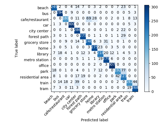 |
|---|
| Fig 1. Confusion matrix for the GBM evaluated on the development dataset. |
The CNN model attains 79.9% (an improvement of 5.1% over the MLP baseline) and the resulting confusion matrix yielded by this model can be seen in Fig 2.
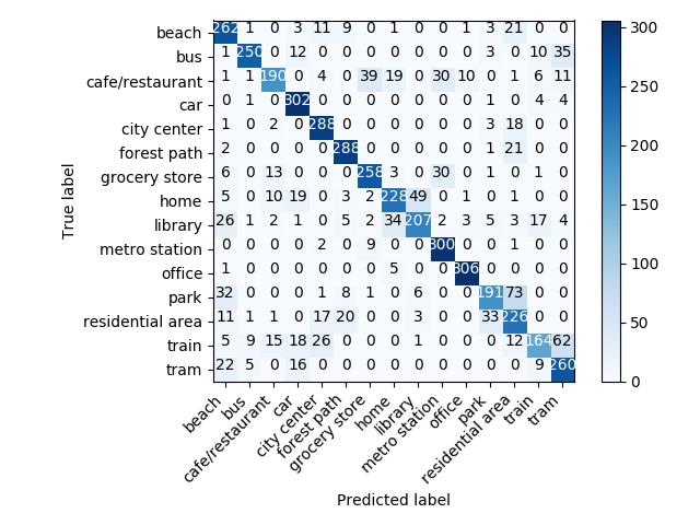 |
|---|
| Fig 2. Confusion matrix for the CNN evaluated on the development dataset. |
Considering the results above, we wanted to see how different the two presented approaches were behaving in terms of predictions and mistakes. To this end, in Fig 3 we plot the difference between:
- the confusion matrix yielded by the GBM (Fig. 1), and
- the confusion matrix yielded by the CNN (Fig. 2) (in this particular order).
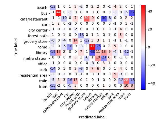 |
|---|
| Fig 3. Difference between the confusion matrixes produced by i) the GBM and ii) the CNN models (in this order), evaluated on the development dataset. |
The plot of Fig 3 can be explained as follows. Along the main diagonal:
- positive numbers illustrate that the GBM model achieves more correct predictions
- negative numbers illustrate that the CNN model achieves more correct predictions
The non-zero values along the diagonal indicate that each model appears to perform better for a determined set of acoustic scenes. For instance, the GBM model performs better in some transportation modes (e.g., bus, train and tram) and in some indoor-quiet enviroments (e.g., home and library). On the contrary, the CNN model is best performing at metro station and achieves slightly better predictions in some environmental contexts (e.g., beach and forest path) or public spaces (e.g., cafe/restaurant and grocery store).
These interesting results should be further analyzed to find out why a model specializes in recogniting a specific set of acoustic scenes. If you have an idea or wish to start a discussion about it, do not hesitate to create and issue or mail me to eduardo.fonseca@upf.edu :)
Then, off the diagonal:
- positive numbers illustrate that the GBM model presents greater confusion for the pairs of acoustic scenes
- negative numbers illustrate that the CNN model presents greater confusion for the pairs of acoustic scenes
By looking at the non-zero values off the diagonal, we can now see that the models get confused between different pairs of acoustic scenes. For examples, the CNN model confuses bus with tram, whereas the GBM model confuses cafe/restaurant with grocery store.
In light of the above, we can summarize saying that both models present different behaviour to some extent, i.e., they are producing a few different predictions, which may be complementary.
To analyse the complementarity of both models we have done a late fusion of the predictions by the two models. We tried very simple combinations of the predictions obtained by each model, namely geometric and arithmetic mean (no learning involved). The arithmetic mean provided the best results. The final system obtained by late fusion of the GBM and CNN attains a classification accuracy of 83.0% on the development set (outperforming the MLP baseline by 8.2%). The confusion matrix yielded by this final system can be seen in Fig 4.
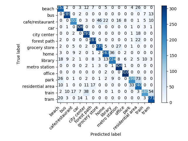 |
|---|
| Fig 4. Confusion matrix for the final system (late fusion of GBM and CNN) evaluated on the development dataset. |